

With the evolving digital panorama, a wealth of information is being generated and captured from numerous sources. Whereas immensely invaluable, this huge universe of data usually displays the imbalanced distribution of real-world phenomena. The issue of imbalanced information will not be merely a statistical problem; it has far-reaching implications for the accuracy and reliability of the data-driven fashions.
Take, for instance, the ever-growing and prevalent concern of fraud detection within the monetary business. As a lot as we need to keep away from fraud on account of its extremely damaging nature, machines (and even people) inevitably have to be taught from the examples of fraudulent transactions (albeit uncommon) to tell apart them from the variety of every day legit transactions.
This imbalance in information distribution between fraudulent and non-fraudulent transactions poses vital challenges for the machine-learning fashions geared toward detecting such anomalous actions. With out acceptable dealing with of the information imbalance, these fashions threat changing into biased towards predicting transactions as legit, doubtlessly overlooking the uncommon cases of fraud.
Healthcare is one other subject the place machine studying fashions are leveraged to foretell imbalanced outcomes, akin to illnesses like most cancers or uncommon genetic problems. Such outcomes happen far much less regularly than their benign counterparts. Therefore, the fashions educated on such imbalanced information are extra vulnerable to incorrect predictions and diagnoses. Such missed well being alert defeats the aim of the mannequin within the first place, i.e., to detect early illness.
These are just some cases highlighting the profound impression of information imbalance, i.e., the place one class considerably outnumbers the opposite. Oversampling and Undersampling are two commonplace information preprocessing methods to steadiness the dataset, of which we’ll deal with undersampling on this article.
Allow us to focus on some common strategies for undersampling a given distribution.
Let’s begin with an illustrative instance to know the importance of under-sampling methods higher. The next visualization demonstrates the impression of the relative amount of factors per class, as executed by a Help Vector Machine with a linear kernel. The under code and plots are referred from the Kaggle pocket book.
import matplotlib.pyplot as plt
from sklearn.svm import LinearSVC
import numpy as np
from collections import Counter
from sklearn.datasets import make_classification


def create_dataset(
    n_samples=1000, weights=(0.01, 0.01, 0.98), n_classes=3, class_sep=0.8, n_clusters=1
):
    return make_classification(
        n_samples=n_samples,
        n_features=2,
        n_informative=2,
        n_redundant=0,
        n_repeated=0,
        n_classes=n_classes,
        n_clusters_per_class=n_clusters,
        weights=listing(weights),
        class_sep=class_sep,
        random_state=0,
    )


def plot_decision_function(X, y, clf, ax):
    plot_step = 0.02
    x_min, x_max = X[:, 0].min() - 1, X[:, 0].max() + 1
    y_min, y_max = X[:, 1].min() - 1, X[:, 1].max() + 1
    xx, yy = np.meshgrid(
        np.arange(x_min, x_max, plot_step), np.arange(y_min, y_max, plot_step)
    )

    Z = clf.predict(np.c_[xx.ravel(), yy.ravel()])
    Z = Z.reshape(xx.form)
    ax.contourf(xx, yy, Z, alpha=0.4)
    ax.scatter(X[:, 0], X[:, 1], alpha=0.8, c=y, edgecolor="ok")


fig, ((ax1, ax2), (ax3, ax4)) = plt.subplots(2, 2, figsize=(15, 12))

ax_arr = (ax1, ax2, ax3, ax4)
weights_arr = (
    (0.01, 0.01, 0.98),
    (0.01, 0.05, 0.94),
    (0.2, 0.1, 0.7),
    (0.33, 0.33, 0.33),
)
for ax, weights in zip(ax_arr, weights_arr):
    X, y = create_dataset(n_samples=1000, weights=weights)
    clf = LinearSVC().match(X, y)
    plot_decision_function(X, y, clf, ax)
    ax.set_title("Linear SVC with y={}".format(Counter(y)))
The code above generates plots for 4 completely different distributions ranging from a extremely imbalanced dataset with one class dominating 97% of the cases. The second and third plots have 93% and 69% of the cases from a single class, respectively, whereas the final plot has a superbly balanced distribution, i.e., all three courses contribute a 3rd of the cases. Plots of the datasets from essentially the most imbalanced to the least are displayed under. Upon becoming SVM over this information, the hyperplane within the first plot (extremely imbalanced) is pushed to a aspect of the chart, primarily as a result of the algorithm treats every occasion equally, no matter the category, and tries to separate the courses with most margin. Therefore, a majority yellow inhabitants close to the middle pushes the hyperplane to the nook, making the algorithm misclassify the minority courses.
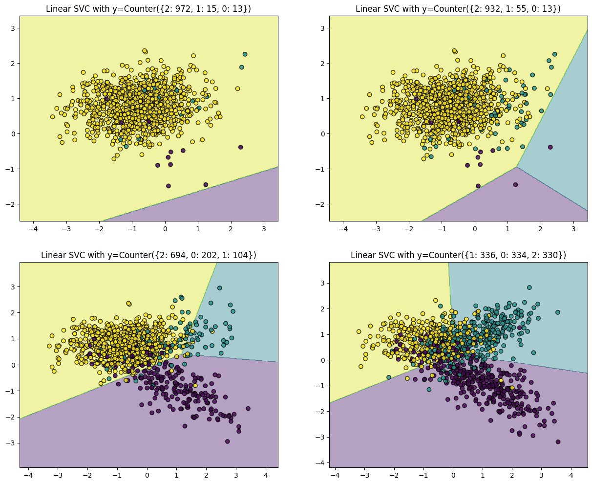
The algorithm efficiently classifies all curiosity courses as we transfer in direction of a extra balanced distribution.
In abstract, when a dataset is dominated by one or just a few courses, the ensuing answer usually leads to a mannequin with greater misclassifications. Nevertheless, the classifier reveals diminishing bias because the distribution of observations per class approaches an excellent break up.
On this case, undersampling the yellow factors presents the only answer to handle mannequin errors originating from the issue of uncommon courses. It is price noting that not all datasets encounter this difficulty, however for those who do, rectifying this imbalance kinds a vital preliminary step in modeling the information.
We’ll use the Imbalanced-Study Python library (imbalanced-learn or imblearn). We will set up it utilizing pip:
pip set up -U imbalanced-learn
Allow us to focus on and experiment with a few of the hottest undersampling methods. Suppose you will have a binary classification dataset the place class ‘0’ considerably outnumbers class ‘1’.
NearMiss Undersampling
NearMiss is an undersampling approach that reduces the variety of majority samples nearer to the minority class. This may facilitate clear classification by any algorithm utilizing area separation or splitting the dimensional area between the 2 courses. There are three variations of NearMiss:
NearMiss-1: Majority class samples with a minimal common distance to the three closest minority class samples.
NearMiss-2: Majority class samples with a minimal common distance to 3 furthest minority class samples.
NearMiss-3: Majority class samples with minimal distance to every minority class pattern.
Let’s exhibit the NearMiss-1 undersampling algorithm by a code instance:
# Import obligatory libraries and modules
import numpy as np
import matplotlib.pyplot as plt
from collections import Counter
from sklearn.datasets import make_classification
from imblearn.under_sampling import NearMiss

# Generate the dataset with completely different class weights
options, labels = make_classification(
    n_samples=1000,
    n_features=2,
    n_redundant=0,
    n_clusters_per_class=1,
    weights=[0.95, 0.05],
    flip_y=0,
    random_state=0,
)

# Print the distribution of courses
dist_classes = Counter(labels)
print("Earlier than Undersampling:")
print(dist_classes)

# Generate a scatter plot of cases, labeled by class
for class_label, _ in dist_classes.gadgets():
    cases = np.the place(labels == class_label)[0]
    plt.scatter(options[instances, 0], options[instances, 1], label=str(class_label))
plt.legend()
plt.present()

# Arrange the undersampling methodology
undersampler = NearMiss(model=1, n_neighbors=3)

# Apply the transformation to the dataset
options, labels = undersampler.fit_resample(options, labels)

# Print the brand new distribution of courses
dist_classes = Counter(labels)
print("After Undersampling:")
print(dist_classes)

# Generate a scatter plot of cases, labeled by class
for class_label, _ in dist_classes.gadgets():
    cases = np.the place(labels == class_label)[0]
    plt.scatter(options[instances, 0], options[instances, 1], label=str(class_label))
plt.legend()
plt.present()
Change model=1 to model=2 or model=3 within the NearMiss() class to make use of the NearMiss-2 or NearMiss-3 undersampling algorithm.
NearMiss-2 selects cases on the core of the overlap area between the 2 courses. With the NeverMiss-3 algorithm, we observe that each occasion within the minority class, which overlaps with the bulk class area, has as much as three neighbors from the bulk class. The attribute n_neighbors within the code pattern above defines this.
This methodology begins by contemplating a subset of the bulk class as noise. Then, it makes use of a 1-Nearest Neighbor algorithm to categorise cases. If an occasion from the bulk class is misclassified, it is included within the subset. The method continues till no extra cases are included within the subset.
from imblearn.under_sampling import CondensedNearestNeighbour

cnn = CondensedNearestNeighbour(random_state=42)
X_res, y_res = cnn.fit_resample(X, y)
Tomek Hyperlinks are intently positioned pairs of opposite-class cases. Eradicating the cases of the bulk class of every pair will increase the area between the 2 courses, facilitating the classification course of.
from imblearn.under_sampling import TomekLinks

tl = TomekLinks()
X_res, y_res = tl.fit_resample(X, y)

print('Authentic dataset form:', Counter(y))
print('Resample dataset form:', Counter(y_res))
With this, we have now delved into the important facets of undersampling methods in Python, overlaying three distinguished strategies: Close to Miss Undersampling, Condensed Nearest Neighbour, and Tomek Hyperlinks Undersampling.
Undersampling is an important information processing step to handle class imbalance issues in machine studying and likewise helps enhance the mannequin efficiency and equity. Every of those methods provides distinctive benefits and might be tailor-made to particular datasets and the objectives of machine studying initiatives.
This text offers a complete understanding of the undersampling strategies and their software in Python. I hope it lets you make knowledgeable choices on tackling class imbalance challenges in your machine-learning initiatives.
Vidhi Chugh is an AI strategist and a digital transformation chief working on the intersection of product, sciences, and engineering to construct scalable machine studying programs. She is an award-winning innovation chief, an creator, and a world speaker. She is on a mission to democratize machine studying and break the jargon for everybody to be part of this transformation.