

Picture by Writer
Linear regression is the basic supervised machine studying algorithm for predicting the continual goal variables primarily based on the enter options. Because the identify suggests it assumes that the connection between the dependant and impartial variable is linear. So if we attempt to plot the dependent variable Y in opposition to the impartial variable X, we are going to get hold of a straight line. The equation of this line might be represented by:
The place,
- Y Predicted output.
- X = Enter function or function matrix in a number of linear regression
- b0 = Intercept (the place the road crosses the Y-axis).
- b1 = Slope or coefficient that determines the road’s steepness.
The central concept in linear regression revolves round discovering the best-fit line for our information factors in order that the error between the precise and predicted values is minimal. It does so by estimating the values of b0 and b1. We then make the most of this line for making predictions.
You now perceive the speculation behind linear regression however to additional solidify our understanding, let’s construct a easy linear regression mannequin utilizing Scikit-learn, a preferred machine studying library in Python. Please observe alongside for a greater understanding.
1. Import Essential Libraries
First, you have to to import the required libraries.
import os
import pandas as pd
import numpy as np
import matplotlib.pyplot as plt
from sklearn.linear_model import LinearRegression
from sklearn.preprocessing import StandardScaler
from sklearn.metrics import mean_squared_error
2. Analyzing the Dataset
You’ll find the dataset right here. It incorporates separate CSV recordsdata for coaching and testing. Let’s show our dataset and analyze it earlier than continuing ahead.
# Load the coaching and check datasets from CSV recordsdata
prepare = pd.read_csv('prepare.csv')
check = pd.read_csv('check.csv')

# Show the primary few rows of the coaching dataset to grasp its construction
print(prepare.head())
Output:
prepare.head()
The dataset incorporates 2 variables and we need to predict y primarily based on the worth x.
# Verify details about the coaching and check datasets, comparable to information varieties and lacking values
print(prepare.information())
print(check.information())
Output:
RangeIndex: 700 entries, 0 to 699
Knowledge columns (whole 2 columns):
 #   Column  Non-Null Depend  Dtype
---  ------  --------------  -----
 0   x       700 non-null    float64
 1   y       699 non-null    float64
dtypes: float64(2)
reminiscence utilization: 11.1 KB


RangeIndex: 300 entries, 0 to 299
Knowledge columns (whole 2 columns):
 #   Column  Non-Null Depend  Dtype
---  ------  --------------  -----
 0   x       300 non-null    int64
 1   y       300 non-null    float64
dtypes: float64(1), int64(1)
reminiscence utilization: 4.8 KB
The above output exhibits that we now have a lacking worth within the coaching dataset that may be eliminated by the next command:
Additionally, examine in case your dataset incorporates any duplicates and take away them earlier than feeding it into your mannequin.
duplicates_exist = prepare.duplicated().any()
print(duplicates_exist)
Output:
2. Preprocessing the Dataset
Now, put together the coaching and testing information and goal by the next code:
#Extracting x and y columns for prepare and check dataset
X_train = prepare['x']
y_train = prepare['y']
X_test = check['x']
y_test = check['y']
print(X_train.form)
print(X_test.form)
Output:
You may see that we now have a one-dimensional array. Whilst you may technically use one-dimensional arrays with some machine studying fashions, it isn’t the most typical observe, and it might result in surprising habits. So, we are going to reshape the above to (699,1) and (300,1) to explicitly specify that we now have one label per information level.
X_train = X_train.values.reshape(-1, 1)
X_test = X_test.values.reshape(-1,1)
When the options are on completely different scales, some might dominate the mannequin’s studying course of, resulting in incorrect or suboptimal outcomes. For this goal, we carry out the standardization in order that our options have a imply of 0 and a normal deviation of 1.
Earlier than:
print(X_train.min(),X_train.max())
Output:
Standardization:
scaler = StandardScaler()
scaler.match(X_train)
X_train = scaler.remodel(X_train)
X_test = scaler.remodel(X_test)
print((X_train.min(),X_train.max())
Output:
(-1.72857469859145, 1.7275858114641094)
We at the moment are carried out with the important information preprocessing steps, and our information is prepared for coaching functions.
4. Visualizing the Dataset
It is essential to first visualize the connection between our goal variable and have. You are able to do this by making a scatter plot:
# Create a scatter plot
plt.scatter(X_train, y_train)
plt.xlabel('X')
plt.ylabel('Y')
plt.title('Scatter Plot of Prepare Knowledge')
plt.grid(True)  # Allow grid
plt.present()
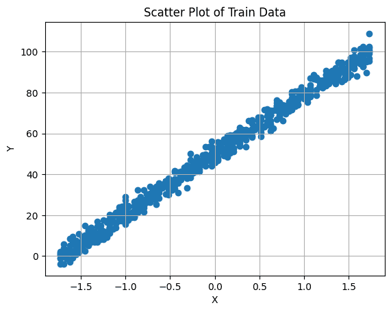
Picture by Writer
5. Create and Prepare the Mannequin
We’ll now create an occasion of the Linear Regression mannequin utilizing Scikit Be taught and attempt to match it into our coaching dataset. It finds the coefficients (slopes) of the linear equation that most closely fits your information. This line is then used to make the predictions. Code for this step is as follows:
# Create a Linear Regression mannequin
mannequin = LinearRegression()

# Match the mannequin to the coaching information
mannequin.match(X_train, y_train)

# Use the skilled mannequin to foretell the goal values for the check information
predictions = mannequin.predict(X_test)

# Calculate the imply squared error (MSE) because the analysis metric to evaluate mannequin efficiency
mse = mean_squared_error(y_test, predictions)
print(f'Imply squared error is: {mse:.4f}')
Output:
Imply squared error is: 9.4329
6. Visualize the Regression Line
We are able to plot our regression line utilizing the next command:
# Plot the regression line
plt.plot(X_test, predictions, coloration="pink", linewidth=2, label="Regression Line")

plt.xlabel('X')
plt.ylabel('Y')
plt.title('Linear Regression Mannequin')
plt.legend()
plt.grid(True)
plt.present()
Output:
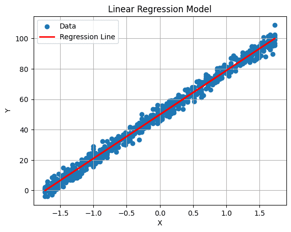
Picture by Writer
That is a wrap! You’ve got now efficiently applied a basic Linear Regression mannequin utilizing Scikit-learn. The abilities you have acquired right here might be prolonged to deal with advanced datasets with extra options. It is a problem price exploring in your free time, opening doorways to the thrilling world of data-driven problem-solving and innovation.
Kanwal Mehreen is an aspiring software program developer with a eager curiosity in information science and purposes of AI in medication. Kanwal was chosen because the Google Technology Scholar 2022 for the APAC area. Kanwal likes to share technical data by writing articles on trending matters, and is keen about enhancing the illustration of ladies in tech business.