Principal Element Evaluation (PCA) with Scikit-Study

In the event you’re accustomed to the unsupervised studying paradigm, you’d have come throughout dimensionality discount and the algorithms used for dimensionality discount such because the principal element evaluation (PCA). Datasets for machine studying sometimes comprise numerous options, however such high-dimensional function areas usually are not at all times useful.

Basically, all of the options are not equally necessary and there are specific options that account for a big share of variance within the dataset. Dimensionality discount algorithms goal to cut back the dimension of the function house to a fraction of the unique variety of dimensions. In doing so, the options with excessive variance are nonetheless retained—however are within the reworked function house. And principal element evaluation (PCA) is without doubt one of the hottest dimensionality discount algorithms.

On this tutorial, we’ll find out how principal element evaluation (PCA) works and methods to implement it utilizing the scikit-learn library.

Earlier than we go forward and implement principal element evaluation (PCA) in  scikit-learn, it’s useful to know how PCA works.

As talked about, principal element evaluation is a dimensionality discount algorithm. That means it reduces the dimensionality of the function house. However how does it obtain this discount?

The motivation behind the algorithm is that there are specific options that seize a big share of variance within the authentic dataset. So it is necessary to seek out the instructions of most variance within the dataset. These instructions are known as principal parts. And PCA is actually a projection of the dataset onto the principal parts.

So how do we discover the principal parts? 

Suppose the info matrix X is of dimensions num_observations x num_features, we carry out eigenvalue decomposition on the covariance matrix of X.

If the options are all zero imply, then the covariance matrix is given by X.T X. Right here, X.T is the transpose of the matrix X. If the options usually are not all zero imply initially, we will subtract the imply of column i from every entry in that column and compute the covariance matrix. It’s easy to see that the covariance matrix is a sq. matrix of order num_features.

Picture by Creator

The primary ok principal parts are the eigenvectors comparable to the ok largest eigenvalues. 

So the steps in PCA could be summarized as follows:
 

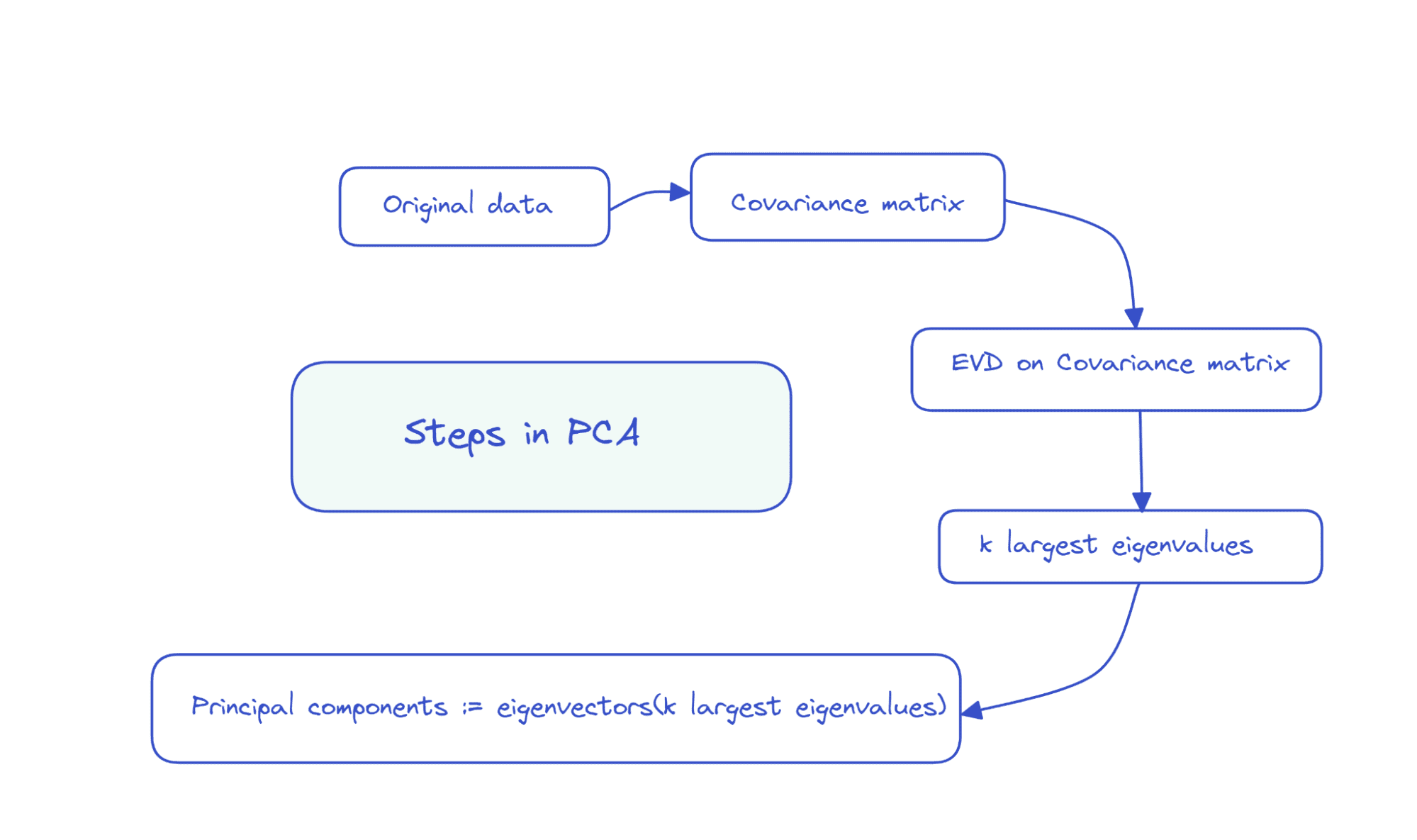
Picture by Creator

As a result of the covariance matrix is a symmetric and optimistic semi-definite, the eigendecomposition takes the next type:

X.T X = D Λ D.T

The place, D is the matrix of eigenvectors and Λ is a diagonal matrix of eigenvalues.

One other matrix factorization approach that can be utilized to compute principal parts is singular worth decomposition or SVD. 

Singular worth decomposition (SVD) is outlined for all matrices. Given a matrix X, SVD of X provides: X = U Σ V.T. Right here, U, Σ, and V are the matrices of left singular vectors, singular values, and proper singular vectors, respectively. V.T. is the transpose of V. 

So the SVD of the covariance matrix of X is given by:
 

We have now the next: 

There are computationally environment friendly algorithms for calculating the SVD of a matrix. The scikit-learn implementation of PCA additionally makes use of SVD below the hood to compute the principal parts.

Now that we’ve realized the fundamentals of principal element evaluation, let’s proceed with the scikit-learn implementation of the identical.

Step 1 – Load the Dataset

To grasp methods to implement principal element evaluation, let’s use a easy dataset. On this tutorial, we’ll use the wine dataset obtainable as a part of scikit-learn’s datasets module.

Let’s begin by loading and preprocessing the dataset:

from sklearn import datasets
wine_data = datasets.load_wine(as_frame=True)
df = wine_data.information

It has 13 options and 178 data in all.

print(df.form)
Output >> (178, 13)

print(df.information())
Output >>

RangeIndex: 178 entries, 0 to 177
Knowledge columns (complete 13 columns):
 #   Column                        Non-Null Rely  Dtype  
---  ------                        --------------  -----  
 0   alcohol                       178 non-null    float64
 1   malic_acid                    178 non-null    float64
 2   ash                           178 non-null    float64
 3   alcalinity_of_ash             178 non-null    float64
 4   magnesium                     178 non-null    float64
 5   total_phenols                 178 non-null    float64
 6   flavanoids                    178 non-null    float64
 7   nonflavanoid_phenols          178 non-null    float64
 8   proanthocyanins               178 non-null    float64
 9   color_intensity               178 non-null    float64
 10  hue                           178 non-null    float64
 11  od280/od315_of_diluted_wines  178 non-null    float64
 12  proline                       178 non-null    float64
dtypes: float64(13)
reminiscence utilization: 18.2 KB
None

Step 2 – Preprocess the Dataset

As a subsequent step, let’s preprocess the dataset. The options are all on completely different scales. To convey all of them to a typical scale, we’ll use the StandardScaler that transforms the options to have zero imply and unit variance:

from sklearn.preprocessing import StandardScaler
std_scaler = StandardScaler()
scaled_df = std_scaler.fit_transform(df)

Step 3 – Carry out PCA on the Preprocessed Dataset

To seek out the principal parts, we will use the PCA class from scikit-learn’s decomposition module.

Let’s instantiate a PCA object by passing within the variety of principal parts n_components to the constructor. 

The variety of principal parts is the variety of dimensions that you just’d like to cut back the function house to. Right here, we set the variety of parts to three.

from sklearn.decomposition import PCA
pca = PCA(n_components=3)
pca.fit_transform(scaled_df)

As a substitute of calling the fit_transform() methodology, you can too name match() adopted by the remodel() methodology.

Discover how the steps in principal element evaluation comparable to computing the covariance matrix, performing eigendecomposition or singular worth decomposition on the covariance matrix to get the principal parts have all been abstracted away after we use scikit-learn’s implementation of PCA.

Step 4 – Inspecting Some Helpful Attributes of the PCA Object

The PCA occasion pca that we created has a number of helpful attributes that assist us perceive what’s going on below the hood.

The attribute components_ shops the instructions of most variance (the principal parts).

Output >>
[[ 0.1443294  -0.24518758 -0.00205106 -0.23932041  0.14199204  0.39466085
   0.4229343  -0.2985331   0.31342949 -0.0886167   0.29671456  0.37616741
   0.28675223]
 [-0.48365155 -0.22493093 -0.31606881  0.0105905  -0.299634   -0.06503951
   0.00335981 -0.02877949 -0.03930172 -0.52999567  0.27923515  0.16449619
  -0.36490283]
 [-0.20738262  0.08901289  0.6262239   0.61208035  0.13075693  0.14617896
   0.1506819   0.17036816  0.14945431 -0.13730621  0.08522192  0.16600459
  -0.12674592]]

We talked about that the principal parts are instructions of most variance within the dataset. However how will we measure how a lot of the overall variance is captured within the variety of principal parts we simply selected?

The explained_variance_ratio_ attribute captures the ratio of the overall variance every principal element captures. Sowe can sum up the ratios to get the overall variance within the chosen variety of parts.

print(sum(pca.explained_variance_ratio_))

Output >> 0.6652996889318527

Right here, we see that three principal parts seize over 66.5% of complete variance within the dataset.

Step 5 – Analyzing the Change in Defined Variance Ratio

We will attempt operating principal element evaluation by various the variety of parts n_components.

import numpy as np
nums = np.arange(14)

var_ratio = []
for num in nums:
  pca = PCA(n_components=num)
  pca.match(scaled_df)
  var_ratio.append(np.sum(pca.explained_variance_ratio_))

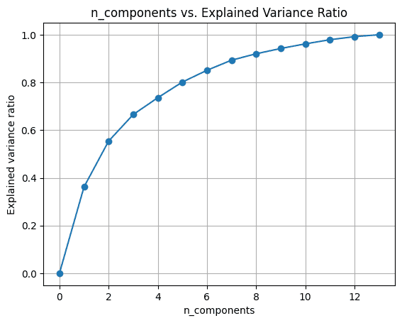
To visualise the explained_variance_ratio_ for the variety of parts, let’s plot the 2 portions as proven:

import matplotlib.pyplot as plt

plt.determine(figsize=(4,2),dpi=150)
plt.grid()
plt.plot(nums,var_ratio,marker="o")
plt.xlabel('n_components')
plt.ylabel('Defined variance ratio')
plt.title('n_components vs. Defined Variance Ratio')

Once we use all of the 13 parts, the explained_variance_ratio_ is 1.0 indicating that we’ve captured 100% of the variance within the dataset. 

On this instance, we see that with 6 principal parts, we’ll have the ability to seize greater than 80% of variance within the enter dataset.
 

I hope you’ve realized methods to carry out principal element evaluation utilizing built-in performance within the scikit-learn library. Subsequent, you’ll be able to attempt to implement PCA on a dataset of your selection. In the event you’re on the lookout for good datasets to work with, take a look at this checklist of web sites to seek out datasets on your information science initiatives.

[1] Computational Linear Algebra, quick.ai
 
 
Bala Priya C is a developer and technical author from India. She likes working on the intersection of math, programming, information science, and content material creation. Her areas of curiosity and experience embrace DevOps, information science, and pure language processing. She enjoys studying, writing, coding, and low! At present, she’s engaged on studying and sharing her data with the developer group by authoring tutorials, how-to guides, opinion items, and extra.